Symbolic Regression 1 of 2

The Promise The Practice and The Paper Review

Symbolic regression is one of those machine learning tasks that we really wish we were good at, but alas, it is a no-go.

Introduction and Motivating Examples

In a nutshell, the goal is to find the ‘simplest’ mathematical formula that fits a data set.

Suppose we had the data $x = \{2, 4, 8, 16\}, y = \{5, 9, 17, 33\},$ then our formula would be $y = 2x + 1$ , which is nice and linear. However, suppose our data were instead the following $x=\{\pi/6, \pi/4, \pi/4 \}, y= \{5/2, \frac{\sqrt{2} + 4}{2}, \frac{\sqrt{3} + 4}{2} \}$ . Then a formula that fits this data perfectly is $y = sin(x) + 2$ . Our formula is simple if we think of $sin$ as an elementary function. If we try to fit a polynomial model to data generated by $y = sin(x) + 2$ then the simplest model without errors would be an infinite series.

Compare this to linear regression in which we fit a linear model to the data or generalizations of linear regression. In a way, symbolic regression is about providing the alphabet letters in the form of symbols and finding the best word to fit our data. Linear regression is about pretending everything is linear, and all errors are normal. So why isn’t symbolic regression more widely used, or at least a more active research topic?

Suppose we had the following python code.

import numpy as np
X = np.random.random((30,5))
y = np.asarray([np.dot(x,x) for x in X])

We see the process that generates $y[0] = X[0]^T \cdot X[0]$ is not linear but is quite simple. The dot product operation is one of the elementary symbols for matrix math. However, if we are not vector operation aware, then the formula is a messy one.

$x_0^2 + x_1^2 +x_2^2 +x_3^2 +x_4^2$

Okay, so maybe we should just include more symbols if this formula looks too complicated. To see why this is a problem, it helps to visualize searching for a symbolic formula as that of looking through a tree.

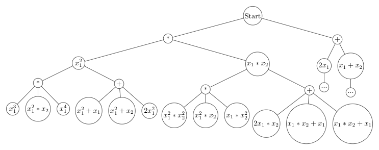
For this tree, let us assume we have only two symbols, multiplication (*) or addition(+). We first choose either addition or multiplication, then we choose which variables to act on. At the start, we only have two variables $x_1 , x_2$ . As we move down the tree, we can think of adding in a ‘new variable’ for our previously performed computation. We can now see the problem. Our tree grows exponentially in-depth, and the more symbols we have, the faster it grows.

Let us reevaluate our example but add in our new dot product operation. To demonstrate some of the issues here, we are going to add in two other variables $x_3, \vec{x}$ . Now we enter the truly tricky territory. What space is our vector operation defined on? Are we only allowed to operate on all of $\vec{x}$ , or can we operate on subsets of our vector $(x_1, x_2), (x_2, x_3), (x_1, x_3), (x_3, x_2)$ or even $(x_1),$ …? If we are allowed to operate on all subsets, then we might as well remove the multiplication symbol, but now we have $2^n$ variables to worry about! Luckily in our example, we only have 8, but most things in life use way more than just three dimensions. Our tree explodes in breadth after only one dot operation. Given that we have a huge unmanageable tree search now, what do we do now?

The Implicit Relaxation Technique

Classically, the way to solve symbolic regression problems was to use evolutionary algorithms. We just use derivative-free optimization, Eureqa! But we live in the age of AI, and those really fancy Neural Network thingies, can’t we do better? One can think of playing chess as a tree search problem as well.

Solving that tree search problem using neural networks is exactly what ‘Deep symbolic regression: Recovering mathematical expressions from data via risk-seeking policy gradients‘ does. But before going into the details of the paper, let’s take two steps back and one forward.

One of the nice things about reinforcement learning (RL) is its compatibility with derivative-free problems. This compatibility is found in the way RL uses rewards. In a classical deep neural network classification problem, one has a loss function that measures how good our classifier is. We then use an automatic differentiation package to compute a gradient relative to our model parameters and minimize our loss function. Vaguely speaking, an RL problem can be thought of as a game of chance where we want to learn a strategy that wins more than it loses. In an RL setting, we replace our loss function with some reward that tells us if we won or lost and how much. We then show our RL algorithm this numerical reward without providing information on the function that generated it. Our algorithm tries to change our strategy, so we win more on average.

Thus for a particular optimization perspective, we have replaced our symbolic regression problem with a relaxation, finding a strategy to ‘win’ at our symbolic regression game more frequently. If we took a loss-based method, we would need to ensure we could compute gradients in terms of our model parameters and our loss function. However, we want to be able to fit expressions such as $sin(x/y) + 3x -y$ and other mathematical functions that have nasty nonlinearities.

Down to the technical Details

Note this section assumes some background in math/RNNs/RL to understand fully but should be 90% comprehensible without said background.

The paper provides a few new ideas and some standard ones from AutoML. First, they use an RNN to generate an autoregressive symbolic expression, or $p( x_i | x_{i-1}, . . . )$ for those of us that need to look up autoregressive. The technique boils down to sampling from an RNN, with a fixed library of outputs $\{ \div, - , *, +, const, x, y, . . . \}$ . Next, we infer where we are in the expression tree and feed in local context symbols along with our state to the RNN. This is a neat trick, as the last output could be very far away from the next location on the expression tree that needs to be filled in, and the local context helps the RNN with the long-term memory issues. They also ensure the expressions are valid by tossing ones that are too short/long, and masking out with zero probabilities for invalid expressions. Invalid expressions include both truly invalid stuff and expressions that are pointless such as $sin(const)$ or $sin(x + cos(x))$ . The first expression is just a silly way of writing constant again, and the latter is excluded by the justification that it “does not appear in virtually any scientific domain.” The last step is to fit the constants employing ‘BFGS.’

The local context trick is new to me, but the other aspects of their RNN process are pretty typical in many AutoML domains. I have definitely seen the same techniques in automatic architecture search for DNNs. I also like that the constants are fitted afterward, which dramatically reduces the complexity of the expression generation task for our RNN.

Next, let’s dig into the fun math! The paper, for the sake of comparing results to other methods, adopts a standard unsquashed reward function called “normalized root-mean-square error’ (NRMSE).

$\frac{1}{\sigma_y}\sqrt{\frac{1}{n} \sum_{i=1}^n (y_i - f(X_i))^2}$

Thus our reward is a modification of mean square error with the notable twist of using the standard deviation $\sigma_y$ of the target values $y_i$ as our normalization factor. Lastly, they perform a squashing operation by $R(\tau) = 1/(1 + NRMSE)$ . From the standpoint of reward engineering for RL, nothing about this really jumps out as insightful or incorrect. Some of the tricks of the trade involve various ways of trying to reshape rewards to make them more or less informative. With their particular squashing operation, one wonders if we are losing the scale of badness. Concretely, if $1 \geq NRMSE$ then our value is in the $[1/2, 1]$ , and $3 \geq NRMSE \geq 1$ maps to $[1/4, 1/2]$ and so on. So when things are very wrong, we only see a slight difference in our reward. This is one of those things that may or may not matter in training, and considering what their second major contribution is ripe for ablation studies.

This second part is a modification to the REINFORCE policy gradient algorithm for RL to increase risk-seeking behavior, which is a weird anthropomorphic way of describing an algorithm that optimizes top quantile behavior instead of mean behavior.

Let us give a short mathematical overview of REINFORCE and then the result. Let $\theta$ be our RNN model parameters, and let $\tau$ be a symbolic expression. Then we write $p(\tau| \theta)$ for the distribution of expressions that our model produces. Improving the quality of our model boils down to improving the expected reward.

$J(\theta) = \mathbb{E}_{\tau \sim p(\tau|\theta)}[R(\tau)]$

$\nabla_{\theta} J(\theta) = \nabla_{\theta}\mathbb{E}_{\tau \sim p(\tau | \theta)} [R(\tau)]$

$= \mathbb{E}_{\tau \sim p(\tau | \theta)} [R(\tau) \nabla_{\theta} \log p(\tau|\theta)]$

The last expression has the crucial property. By this log trick, we can avoid taking the gradient of the expectation, and we are left with a formula that we can approximate by sampling.

$\nabla_{\theta}J(\theta) \approx \frac{1}{N} \sum_{i = 1}^N R(\tau_i) \nabla_{\theta} \log p(\tau_i|\theta)$

Their new objective function is defined in terms of $(1 - \epsilon)$ -quantile with $R_{\epsilon}(\theta)$ the reward of that quantile.

$J(\theta, \epsilon) = \mathbb{E}_{\tau \sim p(\tau | \theta)}[R(\tau) | R(\tau) \geq R{\epsilon}(\theta)]$

$\nabla_{\theta}J(\theta, \epsilon) \approx \frac{1}{\epsilon N}\sum_{i=1}^N [R(\tau_i) - \tilde R_{\epsilon}(\theta)] \mathbf{1}_{R(\tau_i) \geq \tilde R{\epsilon}(\theta)} \nabla_{\theta} \log p(\tau_i| \theta)$

The point of our final equation is that it approximates our gradient by computable elements. A couple of issues arise from this formulation. First, how bad is the estimate of our quantile, and what effect does that have on training? One can see that their prior squashing of the reward can have some nontrivial interaction with the objective function. Lastly, our batch size for updating now depends on $\epsilon$ in a way that will require some hyperparameter optimization as it is not clear that performance does not critically depend on these values.

Further generalization of this objective type could include an exploration factor on the bottom quantile without changing much about the current loss.

Next time we will look a some of the experiments in detail and run some experiments of our own.

Introduction and Motivating Examples

The Implicit Relaxation Technique

Down to the technical Details

Share this:

Related

Leave a comment Cancel reply